Learning a POMDP policy from human demonstrations
Objective
The aim of this project is to learn a belief space policy \(\pi_{\boldsymbol{\theta}}: b \mapsto a\), which takes as input a probability distribution over the state space \(b\) (belief) and outputs an action \(a\), to accomplish a search task given no visual information.
When the state space (robot’s position) is not fully observable it is necessary to represent and consider all hypothetical positions during state estimation and planning in order to act optimally. An optimal control policy can be found by formulating the problem as a Partially Observable Markov Decision Process (POMDP) (the partiality arises from the lack of any visual sensory information) and resolving it via Value Iteration (VI).
This is only feasible when the both the action and state space are discrete which is not naturally the case when considering robotic systems. I propose a method in which a POMDP policy is learned from a set of demonstrations provided by an expert teachers.
Notation and variables
- \(x \in \mathbb{R}^3\), Cartesian position of end-effector.
- \(a \in \mathbb{R}^3 = \dot{x}\), Cartesian velocity of end-effector.
- \(y \in \mathbb{R}^N\), sensory measurement vector.
- \(b := p(x_{t} \lvert a_{1:t},y_{0:t})\), probability distribution over state space.
- \(g : b \mapsto F\), dimensionality reduction, where \(F\) is a feature vector.
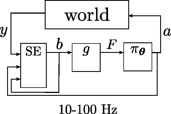
Figure System loop illustrates the interaction between key components which dictates the behavior of the system.

We added between the probability distribution and policy a compression function \(g\). The motivation behind this component is that it is infeasible to directly learn function of \(b\) as it is of high dimensionality. It is thus preferable to compress it to a low dimensional representation whilst retaining most of the information.
\[F = \begin{bmatrix} \hat{x} \\[0.3em] U \\[0.3em] \end{bmatrix} \in \mathbb{R}^4\]- \(\hat{x} = \arg\, \max\limits_{x_t} p(x_{t} \lvert a_{1:t},y_{0:t})\), end-effector’s most likely position.
- \(U = H\left( b \right) \in \mathbb{R}\), entropy.
Task and approach
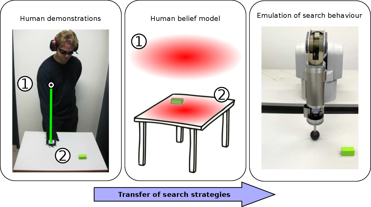
Our approach to learning the belief state control policy for our search task is based on Programming by Demonstration (PbD). In this framework an expert teacher (usually a human) demonstrates to an apprentice (the robot) how to accomplish the task. In this project the task was to search for a wooden block on a table whilst deprived of sight. As such when the human teacher is performing the search task the robot apprentice must infer the teacher’s beliefs such to associate them with his actions in order to reproduce the demonstrated behavior. The Figure below, illustrates the transfer of the search behavior. Before the teacher starts the search his hand is positioned above the table (location #1) and the belief is assumed to be uniform (center illustration, red probability distribution).

Figure: Learning to search from human demonstrations Left: start of the search, the human has his hand located above the table in position #1 and moves his hand downwards to position #2. Center: the belief is initially uniformly distributed (illustrated by the red density) until a contact is made with the table. Right: after inferring the beliefs of the human and observing his actions the robot learns to reproduce the behavior.
The actions of the human teacher were recorded by a vision tracking system (Optitrack) which was also used to infer the tactile and haptic sensations, \(y\). These two components are then used to update the belief following the standard Bayesian recursion. Given that we have access to this information we can proceed to apply the PbD methodology, whose steps are detailed in the section below.
Programming by Demonstration
- Gather a data set of demonstrations from the teacher: \(\mathcal{D} = \{a^{[i]}_{1:T},b^{[i]}_{0:T} \}_{i=1:M}\), where \(i\) is the index of the \(i\)th demonstration (trajectory).
- Compress all recorded beliefs to feature vectors \(F\).
- Learn a generative joint distribution of the actions and compressed beliefs: \(\pi_{\boldsymbol{\theta}}(a,F)\)
- Extract an action from the conditional and use it as a control command for the robot: \(a \sim \pi_{\boldsymbol{\theta}}(a \lvert F)\)
In our setting we used a Gaussian Mixture Model (GMM) as the generative joint distribution:
\[\pi_{\boldsymbol{\theta}}(a,F) = \sum\limits_{k=1}^K w^{[k]} \mathcal{N}([a,F]^{\mathrm{T}};\boldsymbol{\mu},\boldsymbol{\Sigma})\]The parameters \(\boldsymbol{\theta} = \{w^{[k]},\boldsymbol{\mu}^{[k]},\boldsymbol{\Sigma}^{[k]}\}_{1:K}\), are the weights, means and covariances of the individual Gaussian functions, \(\mathcal{N}\). The number of Gaussian components was chosen via model selection with the Bayesian Information Criterion (BIC) and the fitting of the parameters was done with Expectation-Maximisation (EM).
1. Gather teacher demonstrations
A human teacher gives a demonstration on how to achieve the task (find the wooden green block on the table) given
that he is blindfolded.
The position of the teacher’s hand is recorded with an vision tracking system (I was using Optitrack). The sensations the human perceives are inferred from the geometric relation of his hand with a model of the environment which is known a priori.
From multiple demonstrated searches a dataset \(\mathcal{D}\) is obtained from which a generative GMM model is learned.
3. Learn generative distribution and extract actions
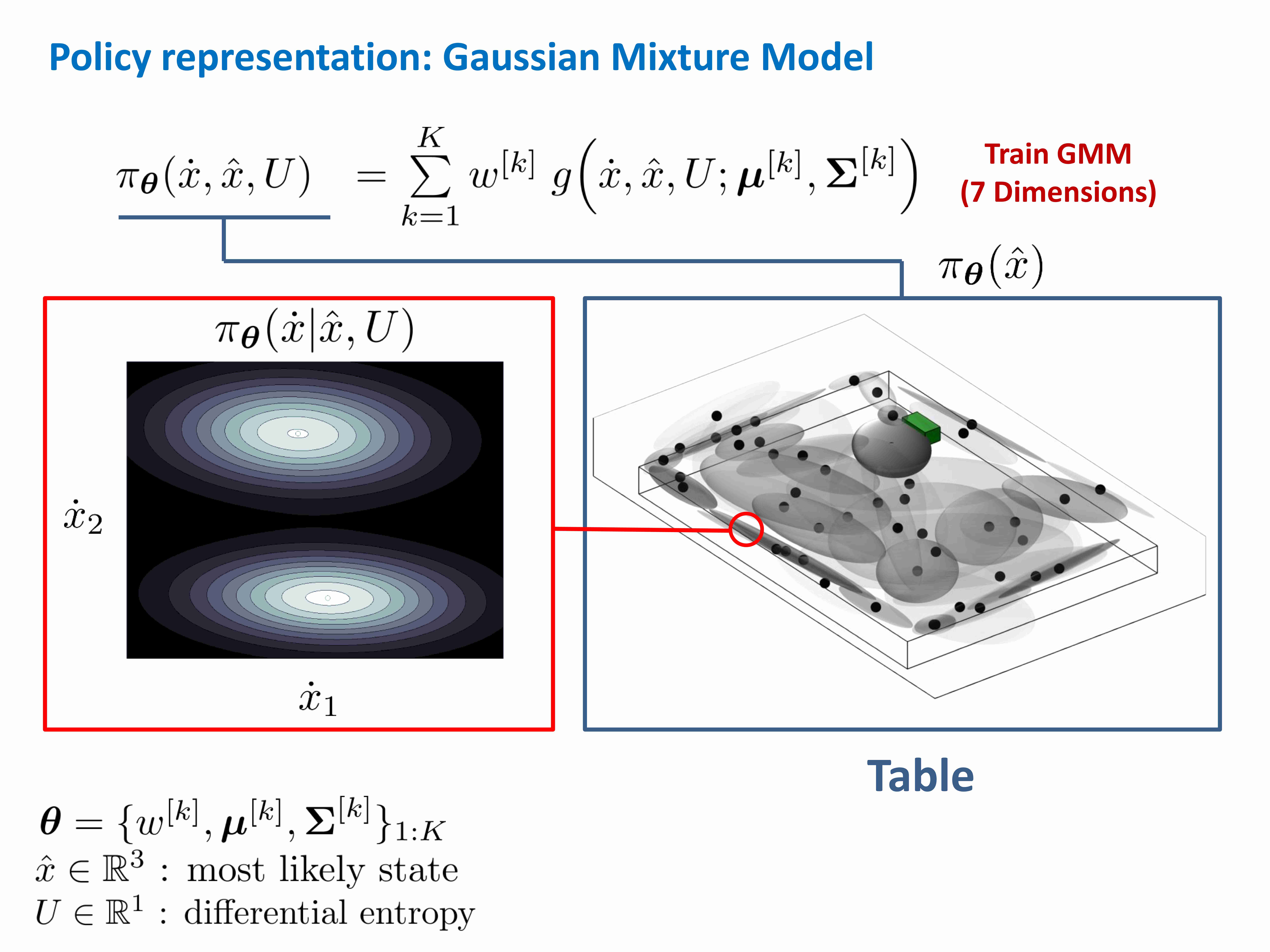
Figure GMM Policy illustrates the marginal distribtion of the GMM model after the number of components was selected via the Bayesian Information Criterion (BIC).

When the GMM joint distribution \(\pi_{\boldsymbol{\theta}}(\dot{x},\hat{x},U)\) is conditioned on the belief state \(F = [\hat{x},U]^{\mathrm{T}}\), it becomes a distribution over actions \(\pi_{\boldsymbol{\theta}}(\dot{x} \lvert \hat{x},U)\). One way of choosing a control velocity to apply is to take the expectation of this distribution \(\dot{x} = \mathbb{E}\{ \pi_{\boldsymbol{\theta}}(\dot{x} \lvert \hat{x},U) \}\). Taking the expectation of the conditional is known as Gaussian Mixture Regression (GMR). Video GMR illustrated the behaviour of GMR on a pac-man agent positioned on top of the table.
Video: Gaussian Mixture Regression (GMR): A pac-man agent is following the actions given by GMR. Left: In blue are the first and second standard deviations of the Gaussian functions of the GMM model. Right: Distribution over velocities, the heading of pac-man agent corresponds to the mean of this distribution.
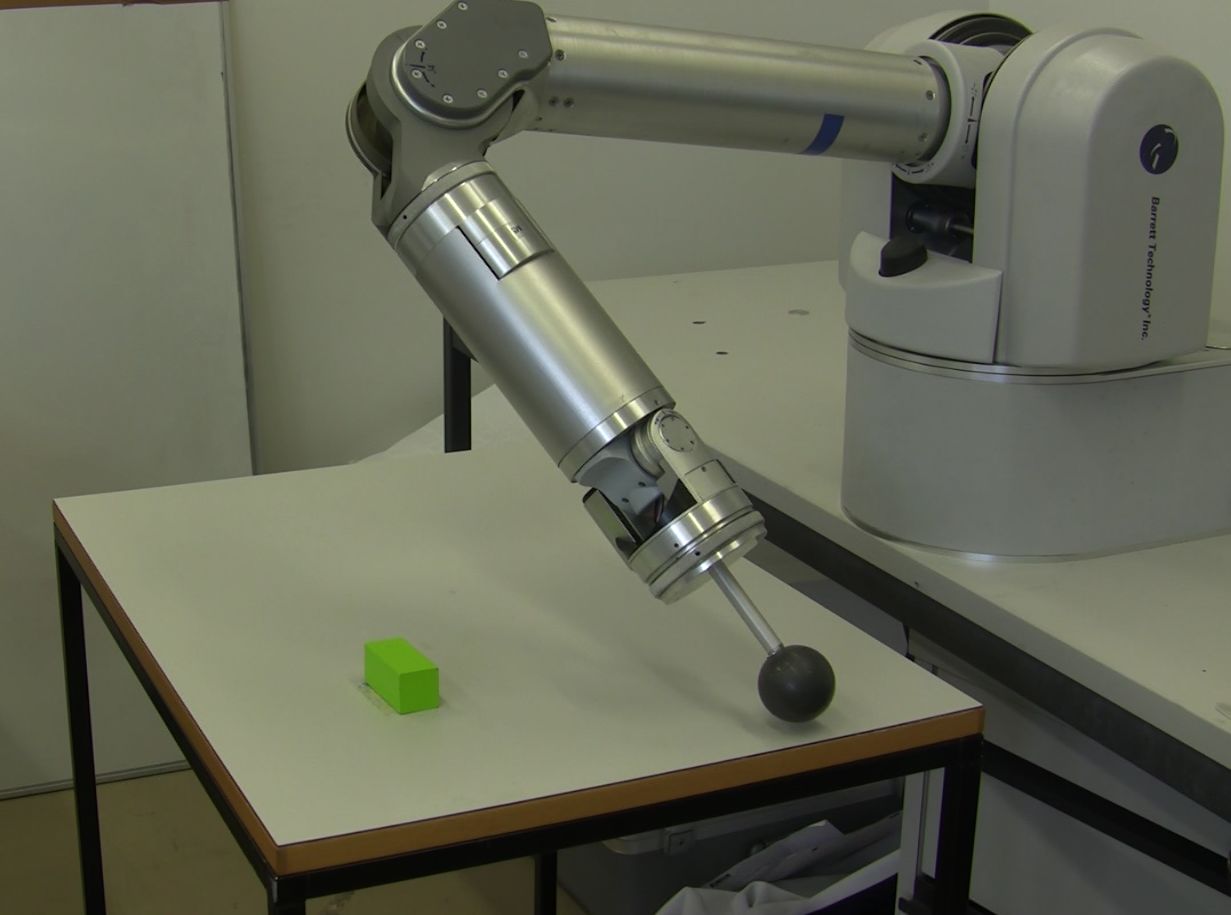
A similar GMR controller was applied for the reproduction of the behaviour demonstrated by the teachers for the block-table search task. Video POMDP Policy illustrates the behaviour the end-effector of a robot would follow.
Video: POMDP GMM policy: GMM model of search strategies learned from human teachers. The white ball represents the true position of the end-effector whilst the blue ball represents the most likely state. The arrows represent different behaviours which can be selected. The cloud of points are part of a the particle filter representing the spatial location belief of both teacher and robot.

