Jacobian

This is a set of notes regarding the Jacobian matrix of robot manipulator. I will be using material for the following references

• Introduction to Robotics Mechanics and Control [1]

• Khatib Introdction to robotics Chapter 4. [2]

• ETHZ Rbot Dynamics lecture notes [3]

It is an important consept and is used in various mappings between joint and cartesian space. There are predominantly two types of Jacobians

• Analytical Jacobian
• Geometric Jacobian

Analytical jacobian

The analytical Jacobian relates the rate of change of joints $\delta q$ to those of the end-effector \(\chi_e\). This relation can be found by linearizing the forward kinematic equation of the manipulator:

\[\chi_e + \delta \chi_e = \chi_e(q + \delta q) = \chi_e(q) + \frac{\partial \chi_e(q)}{\partial q} \delta q + O(\delta q^2)\]

which results in the first order approximation:

\[\delta \chi_e \approx \frac{\partial \chi_e(q)}{\partial q} = J_{e}(q)\delta q\]

where \(4J_{e}(q)\) is the \(m \times n\) analytical Jacobian matrix. By dividing both sides by \(\delta t\) we can an exact relationship between the joint velocitie and end-effector velocities:

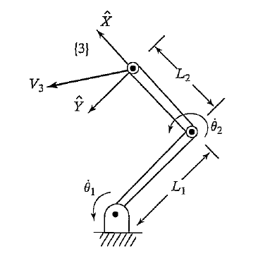
\[\dot{\chi}_e = J_e(q) \dot{q}\]

Next is an example of derivation of the analytical Jacobian for a two link planar manipulator:

Small notatiom notes before continuing:

• \(c_1 = cos(\theta_1)\), the letter indicates if it is sin or cos and the number corresponds to the joint angle.
• \(c_{12} := cos(\theta_1 + \theta_2)\), etc.

The analytical Jacbian is derivative of the forward kinematic \(\chi_e\). We first need to compute the position and orientation of the end effector with respect to the base frame {0}. First we write the transformations between each link before multiplying them to obtain \(\chi_e\). We use \(\theta\) instead of \(q\) to keep the same notation as in [1].

\[{}^0_1T(\theta_1) = \begin{bmatrix} c_1 & -s_1 & 0 & 0 \\ s_1 & c_1 & 0 & 0 \\ 0 & 0 & 1 & 0 \\ 0 & 0 & 0 & 1 \\ \end{bmatrix}\] \[{}^1_2T(\theta_2) = \begin{bmatrix} c_2 & -s_2 & 0 & l_1 \\ s_2 & c_2 & 0 & 0 \\ 0 & 0 & 1 & 0 \\ 0 & 0 & 0 & 1 \\ \end{bmatrix}\] \[{}^2_3T = \begin{bmatrix} 1 & 0 & 0 & l_2 \\ 0 & 1 & 0 & 0 \\ 0 & 0 & 1 & 0 \\ 0 & 0 & 0 & 1 \\ \end{bmatrix}\] \[{}^0_3T(\theta_1, \theta_2) = {}^0_1T(\theta_1)\,{}^1_2T(\theta_2)\,{}^2_3T = \begin{bmatrix} c_1c_2 - s_1s_2 & -c_1s_2 - s_1c_2 & 0 & c_1c_2l_2 + c_1l_1 - s_1s_2l_2 \\ s_1c_2 + c_1s_2 & -s_2s_1 + c_1c_2 & 0 & s_1c_2l_2 + s_1l_1 + c_1s_2l_2 \\ 0 & 0 & 1 & 0 \\ 0 & 0 & 0 & 1 \\ \end{bmatrix}\] \[\chi_e = {}^0_3T(\theta_1, \theta_2) = \begin{bmatrix} {}^0_3R(\theta_1, \theta_2) & {}^0_3P(\theta_1, \theta_2) \\ 0 & 1 \end{bmatrix}\]

The Analytical Jacobian of the end-effector’s position \(J_p\) is the partial derivative of \({}^0_3P(\theta_1, \theta_2)\) with respect to the joint angles.

\[\begin{bmatrix} \dot{x} \\ \dot{y} \end{bmatrix} = \begin{bmatrix} \frac{\partial P_x}{\partial \theta_1} & \frac{\partial P_x}{\partial \theta_2} \\ \frac{\partial P_y}{\partial \theta_1} & \frac{\partial P_y}{\partial \theta_2} \\ \end{bmatrix}\begin{bmatrix} \dot{\theta}_1 \\ \dot{\theta}_2 \end{bmatrix}\]

For the above exercise:

\[J_p = \begin{bmatrix} -l_1 s_1 - l_2 s_{12} & -l_2 s_{12} \\ l_1 c_1 & l_2 c_{12} \end{bmatrix}\]

The same can be done for the rotation part of \({}^0_3R(\theta_1, \theta_2)\) which will give a \(9 \times 2\) matrix \(J_r\). We do not derivate it here as we will be mostly using the geometric Jacobian.

The analytical Jacobian gives the rate of the chane of the end-effector and not its linear and angular velocity in general. In the case of planar systems, as it is often the case in exercise books, it does give velocities as the analytical and geometric jacbian are the same. This will become apprent when deriving the geometric jacbian.

Computation of end-effector linear and angular velocity

The mapping from joint to end-effector linear and angular velocity can be computed by propergating these quantities from link to link and by adding the velocity compnents generated by each link.

\[{}^{i+1}\omega_{i+1} = {}^{i+1}_iR\,{}^i\omega_i + \dot{\theta}_{i+1} {}^{i+1}\hat{Z}_{i+1}\] \[{}^{i+1}v_{i+1} = {}^{i+1}_iR ({}^iv_i + {}^i\omega_i \times {}^iP_{i+1})\]

The superscript index is for the frame and subscript is for the link. This propergation can be used to derive the geometric Jacobian.

Geometric Jacobian

The geometric Jacobian also known as the Basic or explicit Jacobian maps joint velocities to linear and angular velocities:

\(\begin{pmatrix} v \\ \omega \end{pmatrix} = J_0(q)\dot{q}\).

\[J_0(q) = \begin{pmatrix} \frac{\partial P}{\partial q_1} & \dots & \frac{\partial P}{\partial q_n} \\ {}^{0}z_1 & \dots & {}^{0}z_n \end{pmatrix}\]

where \({}^{0}z_i\) is the 3rd column of the rotation matrix \({}^{0}_iR\), see section 4.7 of [3] and Section 2.8.5 “Geometric or Basic Jacobian” of [2].

Relation between Geometric and Analytical Jacobian

See [2] Section 2.8.6

Jacobian properties

\(\dot{\theta} = J^{-1}(\theta)\,v\): invserse of the Jacobian is required. If there are singularities (loss of full rank) the inverse cannot be commputed.

\(\tau = J^{T}(\theta)\,\mathcal{F}\): Cartesian forces can be converted to torques without having to inverse the Jacobian.