
Point Mass Filter
- Matlab implementation of PMF can be found here: point-mass-filter
The Point Mass Filter (PMF) is the deterministic counter part of the Particle Filter (PF). That is the PMF does not require a re-sampling step. This is advantageous both computational speed and it considerably reduces the black art necessary for tuning the parameters of the PF.
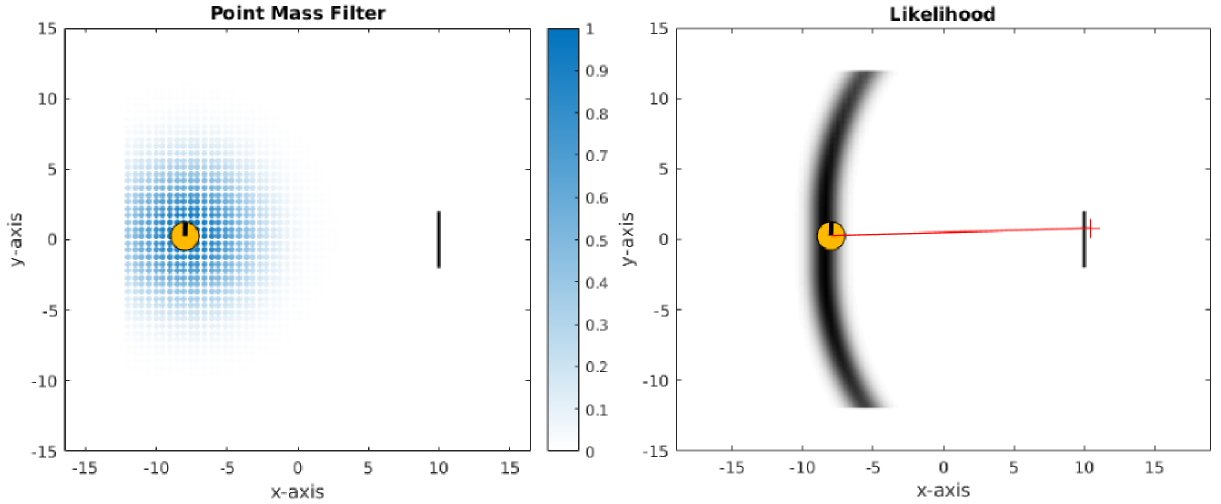
Instead of representing the filtered probability distribution \(p(x_t|y_{0:t},u_{1:t})\) by a set of samples drawn from a proposal distribution, as it is the case for PF, the state space \(x\) is deterministically discretized and represented by a grid. The value of each grid point or cell contains a valid probability in contrast to the PF where a point or particle represents a sample drawn from a proposal distribution as the true probability distribution is unknown. The PMF directly estimates the filtered probability distribution.
Summary of the main differences (pros/cons) of the PMF and PF.
PMF
-
PMF grid values are probabilities whilst the PF particles are samples draw from an proposal distribution. If you wanted to get an estimation of the filtered probability when using a PF, you would have to extract it from the set of particles by either fitting a Gaussian Mixture Model to them (this is one example) or integrate the number of particles within discretized intervals.
-
PMF has no re-sampling step which reduces computation and as a result there is no need to tune the hyper-parameters of a re-sampling kernel (usually a Gaussian) which is necessary for PF.
-
PMF parameters are intuitive. You can set the minimum and maximum resolution of the grid which will dynamically resize as wanted.
-
The PF is straight forward the implement, but hard to tune. The PMF is “harder” to implement but easy to tune.