Fitted Policy Iteration for a POMDPs for a continuous state-action space.

4 minute read

Objective

The parameters of a continuous state and action POMDP policy are initially learned from human teachers and improved through a fitted reinforcement learning approach. As an application we consider the task in which both human teachers and robot apprentice must successfully localize and connect an electrical power socket, a task also known as Peg in hole (PiH), whilst deprived of vision. To accomplish this the following steps are followed:

Gather a dataset of demonstrations of the task (find and connect the power socket).
Learn a value function of the task via fitted reinforcement learning.
Learn the parameters of the POMDP policy whilst weighting the data points by the value function.

A technical report of this project can be downloaded from: here.

Notation and variables

\(x \in \mathbb{R}^3\), Cartesian position of end-effector.
\(a \in \mathbb{R}^3 = \dot{x}\), Cartesian velocity of end-effector.
\(y \in \mathbb{R}^N\), sensory measurement vector.
\(b := p(x_{t} \lvert a_{1:t},y_{0:t})\), probability distribution over state space.
\(g : b \mapsto F\), dimensionality reduction, where \(F\) is a feature vector.

Overview

Following the Programming by Demonstration (PbD) approach, human teachers demonstrate the search and connection task, see Figure Peg-in-hole search task.

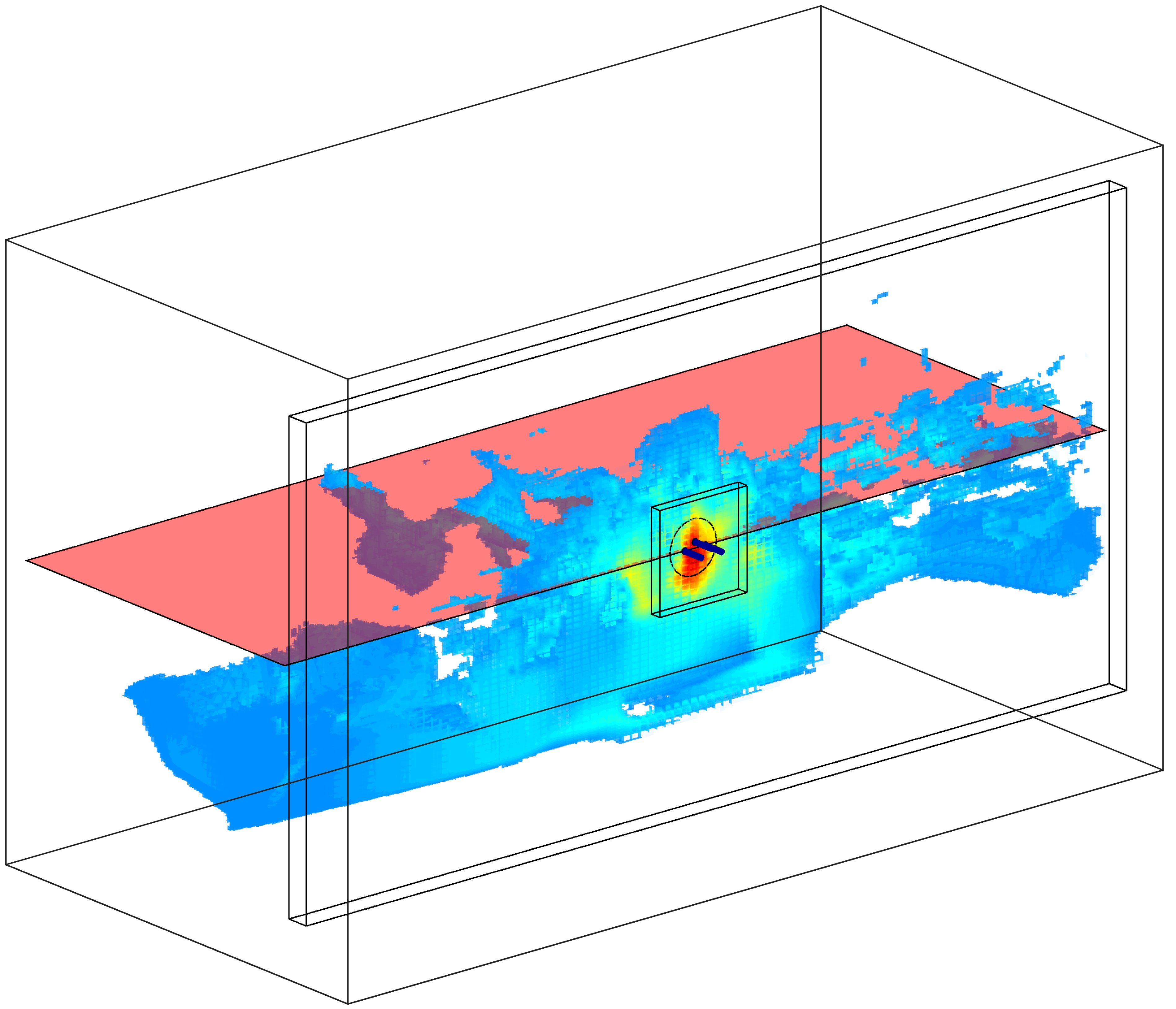
Video: Peg-in-hole search task: A blindfolded human teacher demonstrating the peg-in-hole search task. The holder is equipped with markers and an ATI force/torque sensor from which both velocity and wrench information can be read at every time step.

The tool the teacher is using is a peg holder from which the velocity and wrench can be obtained, with the help of a motion tracking system (Optitrack) and ATI force torque sensor. With both motion (velocity) and sensing information (wrench) we recursively update a Bayesian state space estimation of the peg’s Cartesian position. A position estimation is necessary as both the human teacher and robot apprentice do not have access to any visual information when they have to accomplish the task. Figure Point Mass Filter, illustrated the Bayesian state space estimation obtained through the recursive application of the motion and measurement models.

Video: Point Mass Filter: Given an initially known probability distribution all future distributions obtained via the Bayesian update. The red line represents the path followed by a human teacher.

After learning a value function \(V^{\pi}(F)\) and improving the policy \(\pi_{\boldsymbol{\theta}}: F \mapsto a\) we can successfully transfer the teachers’ behavior to the KUKA LWR robot, see Figure KUKA LWR PiH.

Video: KUKA LWR PiH: Application of the learned POMDP policy.

Fitted Policy Iteration

Fitted Policy Iteration (FPI) is an off-line on-policy Reinforcement Learning (RL) methods which iteratively estimates a value function (policy evaluation) and then uses it to update the parameters of the policy (policy improvement). It is also an Actor-Critic and Batch/Experience replay RL method. The steps of FPI are in essence the same as Policy Iteration where the difference is that we use a Fitted RL approach to learn the value function and an Expectation-Maximisation (EM) to improve the parameters of the policy.

Fitted Policy Evaluation (FPE)

Given a table of state-reward \(\mathcal{D} = \{ (x^{[i]}_{0:T},a^{[i]}_{0:T}) \}_{i=1:M}\) where \(i\) stands for the \(i\)th demonstration (episode). The value function is learned through the repeated application of Bellman’s on-policy backup operator to the dataset,

\[\hat{V}_{k+1}^{\pi}(x) = Regress(x, r + \gamma \hat{V}_{k}^{\pi}(x))\]

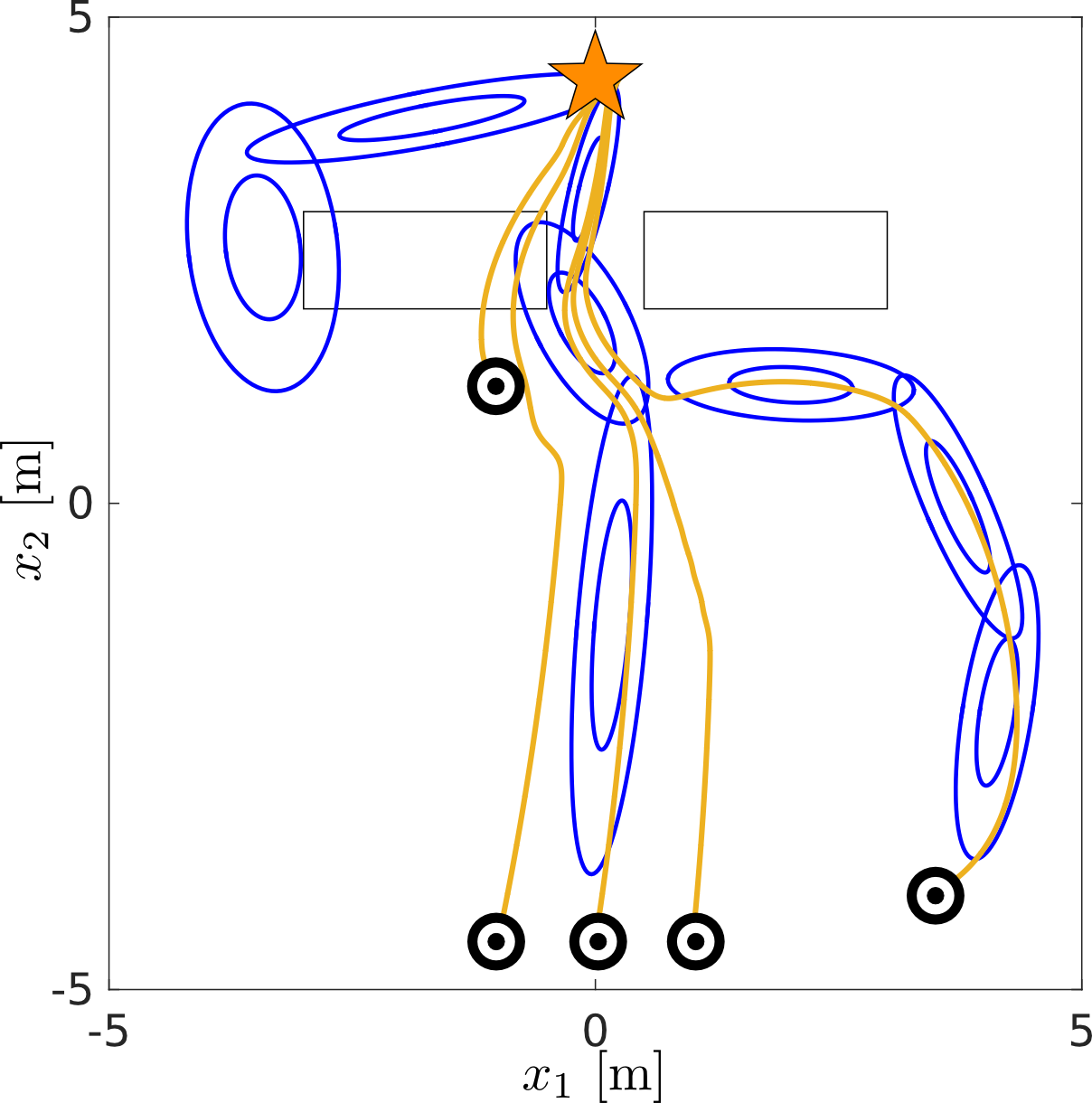
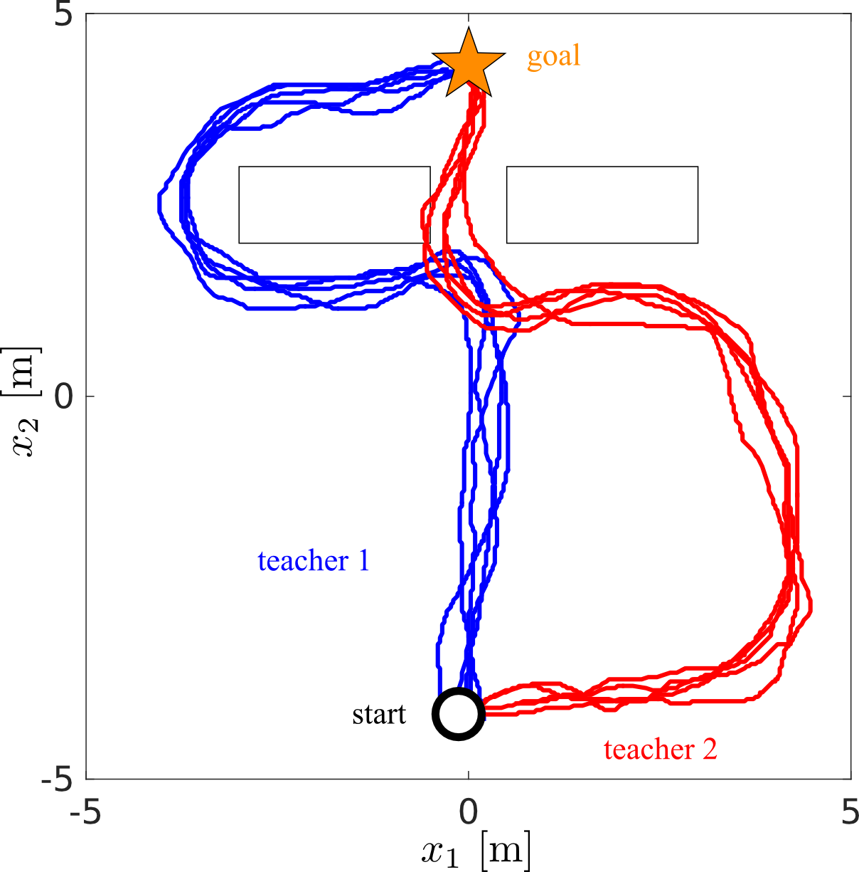
until converges of the bellman residual. Figure 2D teacher demonstrations illustrates a set of demonstrations given by two teachers. The task is reach to goal state (start) given the starting state. Neither teacher demonstrates the optimal solution which is to go in a straight line from start to goal.

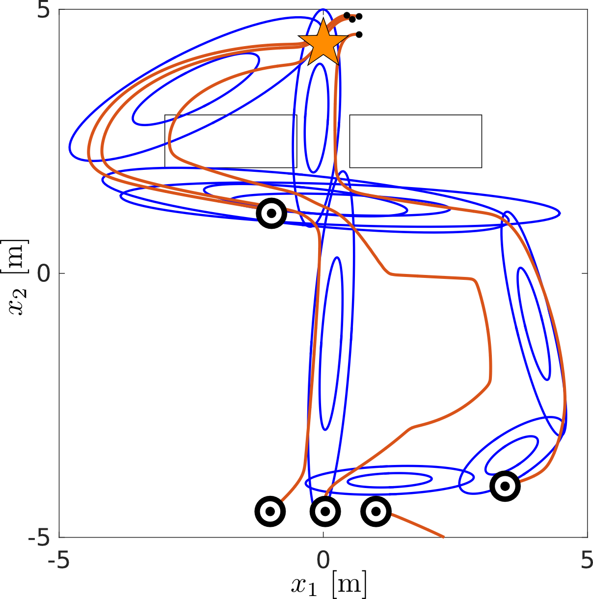
Figure: 2D teacher demonstrations Two teachers demonstrate the task of going form start go goal state. Neither of the two demonstrate the optimal solution, which is to go in a straight path to the goal.

In Figure Fitted Policy Evaluation, the on-policy Bellman equation is repeatably applied to the dataset. At the first time step the target value of the regressor function (which is Locally Weighted Regression) is simply the reward: \(\hat{V}_0^{\pi} : x \mapsto r\). In the second iteration, a new target for the regressor function is computed: \(\hat{V}_1^{\pi} : x \mapsto r + \gamma \hat{V}_0^{\pi}(x)\) which depends on the previous value function estimate.

Video: Fitted Policy Evaluation: At each time iteration: First the target value of the regression is updated, that the bellman value. Second a regression function mapping state to value function is learned. In this case we are using Locally Weighted Regression (LWR).

Policy Improvement

Given the estimate of the value function \(\hat{V}^{\pi}(x)\) we can use it to improve the parameters of the policy, which is a Gaussian Mixture Model (GMM) in our application. This can be achieved my maximizing the logarithmic lower point of the objective function \(J(\boldsymbol{\theta}) = \mathbb{E}\{R\}\) of the task with respect to the policies parameters \(\boldsymbol{\theta}\):

\[\nabla_{\boldsymbol{\theta}} Q(\boldsymbol{\theta},\boldsymbol{\theta}') = \sum\limits_{i=1}^{N}\sum\limits_{t=0}^{T^{[i]}} \nabla_{\boldsymbol{\theta}} \log \pi_{\boldsymbol{\theta}}(x^{[i]}_t,a^{[i]}_t) \mathcal{Q}^{\boldsymbol{\theta}'}(x^{[i]}_t,a^{[i]}_t) \\]